ARCHIVED – Duvernay Resource Assessment – Energy Briefing Note
This page has been archived on the Web
Information identified as archived is provided for reference, research or recordkeeping purposes. It is not subject to the Government of Canada Web Standards and has not been altered or updated since it was archived. Please contact us to request a format other than those available.
Duvernay Resource Assessment – Energy Briefing Note [PDF 4021 KB]
Duvernay Resource Assessment
Energy Briefing Note
September 2017


Copyright/Permission to Reproduce
ISSN 1917-506X
Foreword
National Energy Board
The National Energy Board (NEB or Board) is an independent national energy regulator. Its role is to regulate, among other things, the construction, operation and abandonment of pipelines that cross provincial or international borders, international power lines and designated interprovincial power lines, imports of natural gas and exports of crude oil, natural gas liquids, natural gas, refined petroleum products, and electricity, and oil and gas exploration and production activities in certain areas. The NEB is also charged with providing timely, accurate and objective information and advice on energy matters.
The NEB’s strategic outcome states: The Regulation of pipelines, power lines, energy development and energy trade contributes to the safety of Canadians, the protection of the environment and efficient energy infrastructure and markets, while respecting the rights and interests of those affected by NEB decisions and recommendations.
The Board’s main responsibilities include regulating:
- the construction, operation, and abandonment of pipelines that cross international borders or provincial/territorial boundaries;
- associated pipeline tolls and tariffs;
- the construction and operation of international power lines and designated interprovincial power lines;
- imports of natural gas and exports of crude oil, natural gas, natural gas liquids, refined petroleum products, and electricity; and
- oil and gas exploration and production activities in specified northern and offshore areas.
The Alberta Geological Survey
The Alberta Geological Survey (AGS) is a branch of the Alberta Energy Regulator (AER) and provides geological information and advice to the Government of Alberta, the AER, industry, and the public to support responsible exploration, sustainable development, regulation, and conservation of Alberta's resources.
AGS is responsible for describing the geology and resources in the province, delivering geoscience information and knowledge in several key areas, including surficial mapping, bedrock mapping, geological modelling, resource evaluation (in-place hydrocarbons, minerals), groundwater, and geological hazards. AGS also is responsible for maintaining the Alberta Table of Formations and providing geoscience outreach to stakeholders.
Executive Summary
The NEB, using geology and in-place hydrocarbon information determined by the AGS, has assessed Alberta’s Duvernay Shale for its marketable petroleum potential. The NEB expects that the Duvernay Shale can produce a total of 542 million cubic metres (m³) (3.4 billion barrels) of marketable crude oil, 2.17 trillion m³ (76.6 trillion cubic feet (Tcf)) of marketable gas, and 995 million m³ (6.3 billion barrels) of marketable natural gas liquids (NGLs).
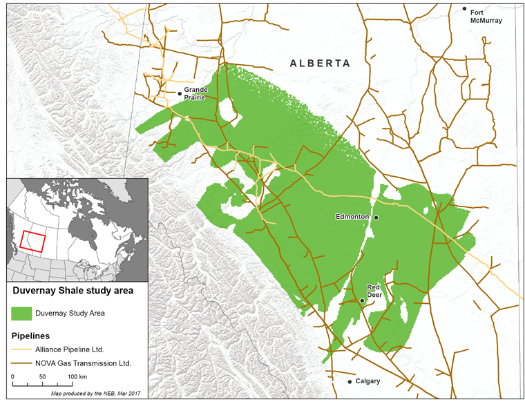
Figure 1. Location of the Duvernay Shale in Alberta and Canada
Description:
This map that shows the location of the Duvernay Shale study area. Calgary, Alberta, is located just south of the study area's southern end while Grande Prairie, Alberta, is located at the study area's northwest end. The figure also shows the gas pipeline systems (Nova Gas Transmission Limited and Alliance Pipeline Limited) that run through the study area.
Since 2011, companies have been testing the Duvernay Shale of Alberta for shale gas and shale oil. The Duvernay extends under 130 000 square kilometres (km²) of Alberta, or 20% of the province (Figure 1). Importantly, the Duvernay Shale is rich in NGLs, including condensateFootnote 1, which is often mixed with bitumen from the Alberta oil sands so the bitumen can be thinned and shipped in oil pipelines.
The Duvernay Shale’s marketable resourcesFootnote 2 are the total amount of sales-quality petroleum that can potentially be recovered from the formation. This is different than the Duvernay Shale’s in-place resourcesFootnote 3,Footnote 4, which measure how much petroleum the formation contains, but do not indicate how much might be produced from it. This is also different than the Duvernay Shale’s reservesFootnote 5, which measure how much petroleum has been discovered close to wells already drilled, but do not estimate how much might be produced from undeveloped areas.
Geological Description
During the Upper Devonian (from 383 million years to 359 million years ago), much of western Canada was flooded by high sea levels. Tall reefs and broad carbonate shelves grew in the tropical climate while mud was deposited in the basins between them. During one stage of reef building about 380 million years ago, the Duvernay Shale was deposited as organic-rich mud between Leduc Formation reefs (Figure 2).
Figure 2. The location of reefs, carbonate shelves, and basins during deposition of the Duvernay ShaleFootnote 6
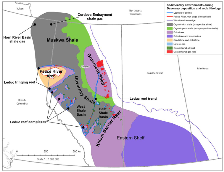
Source: Modified from Atlas of the Western Canada Sedimentary Basin
Description:
This map shows the location of reefs, carbonate shelves, and shale basins during deposition of Alberta's Duvernay Shale. The Duvernay Shale basin of west-central Alberta is bounded in the south by shallow-water carbonates of the Eastern Shelf and on its east by shallow-water carbonates of the Grosmont Shelf. On its northwest side, the Duvernay Shale basin is bounded by reefs that fringed the Peace River Arch. Reef complexes of the Leduc Formation, which grew as platforms surrounded by deep water, are located in the western portion of the Duvernay Shale Basin.
The Duvernay Shale is rich in organic matter and when the formation began to be deeply buried and heated about 100 million years ago, oil and gas were generated. Some of the oil and gas escaped into Leduc Formation reefs, which host some of the largest conventional oil fields in Alberta. Other oil and gas remained in the Duvernay Shale and is now being developed. The Duvernay is related to other prospective shales, such as the Muskwa Shale of northwest Alberta and northeast British Columbia, and the Canol Shale of the Northwest Territories and YukonFootnote 7.
The Duvernay Shale is about 1 km deep at its northeast limit and deepens towards Alberta’s foothills, where it is over 5 km deep. The Duvernay’s net-pay thicknessFootnote 8 ranges from near zero to over 100 m. Formation porosity ranges from about 2 to 10% by volume and its organic content ranges from 2 to 5% by weight. The Duvernay Shale is under-pressured where shallow and over-pressuredFootnote 9 where deep. Because the Duvernay’s geology varies widely, its petroleum volume and contents change depending on location. In particular, shallower areas are oil rich while deeper areas are gas rich. In between these areas, the gas is rich in NGLs, including condensate. For more details on Duvernay geology, please see footnotes 3, 4, and 5.
Methods
The study area was divided into tracts of land 2.6 km² (one square mile) each. Tracts were excluded where the Duvernay was too thin, had too little gas, or had too little pressure to be developed. Production from 96 Duvernay Shale wells was analysed before being grouped to create an index well with a range of potential low to high outcomes. Five index wells, as adjusted to local geology, were assumed to be drilled in each remaining tract to determine recoverable petroleum. Raw gas was converted to marketable gas by removing impurities and subtracting the fuel gas required to power wellsite operations, gas processing, and gas shipping. Field condensate was treated like crude oil.Footnote 10
Assessment Results and Observations
The regionally extensive Duvernay Shale has the potential to produce a total of 2.17 trillion m³ (76.6 Tcf) of marketable gas, 995 million m³ (6.3 billion barrels) of marketable NGLs, and 542 million m³ (3.4 billion barrels) of marketable crude oil (Table 1). The low and high estimates in Table 1 indicate the uncertainty around the expected (average) values. Maps of the expected resources are available in Appendix A. Estimates of individual NGLs (ethane, propane, butane, and pentanes plus) are also included in Table 1. For in-place resources, please see the AGS report in footnote 4.
| Marketable Resource | Metric Gas: trillion m³ Oil and NGLs: billion m³ |
Imperial Gas: Tcf Oil and NGLs: billion barrels |
||||
|---|---|---|---|---|---|---|
| Low | Expected | High | Low | Expected | High | |
| Gas | 0.963 | 2.168 | 3.713 | 34.021 | 76.567 | 131.132 |
| Oil | 263.1 | 542.2 | 895.0 | 1.655 | 3.411 | 5.629 |
| NGLs | 446.7 | 994.6 | 1699.5 | 2.810 | 6.256 | 10.690 |
| Ethane | 241.1 | 539.5 | 922.0 | 1.516 | 3.394 | 5.799 |
| Propane | 116.0 | 257.85 | 440.2 | 0.730 | 1.622 | 2.769 |
| Butane | 57.1 | 126.41 | 215.4 | 0.360 | 0.795 | 1.355 |
| Pentanes plus | 32.3 | 70.81 | 120.14 | 0.203 | 0.456 | 0.756 |
As companies increasingly develop the Duvernay and improve well designs based on what they learn from early results, new wells could perform better than old wells and increase recoveries. Further, some areas in the Duvernay are less explored than other areas (such as the Duvernay’s East Basin) and resources could be discovered in places that were thought to be not prospective. Therefore, the estimates of marketable oil, gas, and NGLs in this study could be conservative.
For perspective, Canada consumes about 89 billion m³ (3.1 Tcf) of natural gas per year and 0.1 billion m³ (0.6 billion barrels) of crude oil. The Montney Formation’s marketable gas resource has been assessed as 12.7 trillion m³ (449 Tcf)Footnote 11, the Liard Basin as 6.2 trillion m³ (219 Tcf))Footnote 12, and the Horn River Basin as 2.2 trillion m³ (78 Tcf).)Footnote 13 The Bakken Formation’s marketable oil resource (Saskatchewan only) is expected to be 0.22 billion m³ (1.4 billion barrels))Footnote 14 and the Montney Formation’s 0.18 billion m³ (1.1 billion barrels). The Montney Formation’s marketable NGLs were estimated to be 2.3 billion m³ (14.5 billion barrels).)Footnote 15
By combining this marketable gas estimate with prior assessments, the total ultimate potential for natural gas in the Western Canada Sedimentary Basin (WCSB) is estimated to be 31.9 trillion m³ (1 128 Tcf) (Table 2). Of this, 26.2 trillion m³ (924 Tcf) remains after cumulative production to year-end 2015 is subtracted. This total is expected to evolve, likely growing over time as additional potential is estimated in unassessed formations. Overall, Canada has a very large remaining natural gas resource base in the WCSB to serve its markets well into the future.
| Area | Gas Type | 109 m³ | Tcf | ||||
|---|---|---|---|---|---|---|---|
| Ultimate Potential | Cumulative Production | Remaining | Ultimate Potential | Cumulative Production | Remaining | ||
| Alberta | Conventional | 6 276 | 4 712 | 8 610 | 221.6 | 166.4 | 313.4 |
| Unconventional | 7 046 | 248.8 | |||||
| CBM portion | 101 | 3.6 | |||||
| Montney portion | 5 042 | 178.1 | |||||
| Duvernay portion | 2 168 | 76.6 | |||||
| Alberta Total | 13 587 | 479.8 | |||||
| British Columbia | Conventional | 1 462 | 811 | 15 505 | 51.6 | 28.6 | 547.6 |
| Unconventional | 14 854 | 524.6 | |||||
| Horn River portion | 2 198 | 77.6 | |||||
| Montney portion | 7 677 | 271.1 | |||||
| Cordova portion | 248 | 8.8 | |||||
| Liard portion | 4 731 | 167.1 | |||||
| British Columbia Total | 16 316 | 576.2 | |||||
| Saskatchewan | Conventional | 297 | 227 | 152 | 10.5 | 8.0 | 5.4 |
| Unconventional | 82 | 2.9 | |||||
| Bakken portion | 82 | 2.9 | |||||
| Saskatchewan Total | 379 | 13.4 | |||||
| Southern NWT | Conventional | 132 | 14 | 1 368 | 4.7 | 0.5 | 48.3 |
| Unconventional | 1 250 | 44.1 | |||||
| Liard portion | 1 250 | 44.1 | |||||
| Southern NWT Total | 1 382 | 48.8 | |||||
| Southern Yukon | Conventional | 61 | 6 | 271 | 2.2 | 0.2 | 9.6 |
| Unconventional | 215 | 7.6 | |||||
| Liard portion | 215 | 7.6 | |||||
| Southern Yukon Total | 276 | 9.8 | |||||
| WCSB Total | 31 941 | 5 770 | 26 172 | 1128 | 204 | 924 | |
| Notes: – Determined from reliable, published assessments by federal and provincial agencies. – Cumulative production is determined from provincial and territorial gas reserves reports. – For this table, “unconventional” is defined as natural gas produced from coal (CBM) or by the application of multi-stage hydraulic fracturing to horizontal wells. – The ultimate potential for natural gas should be considered an estimate that will evolve over time. Additional unconventional potential may be found in unassessed formations. |
|||||||
Appendix A: Resource Maps
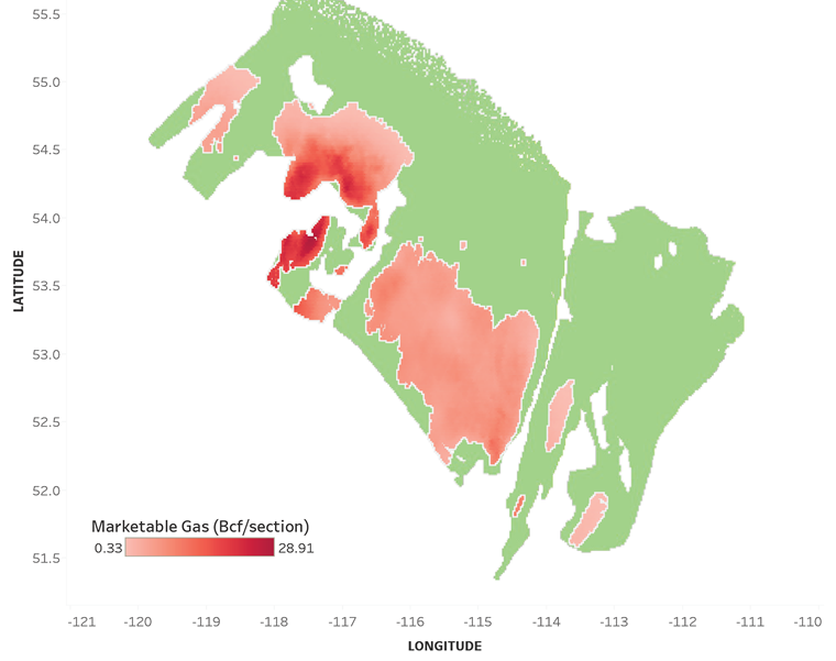
Figure A1. Map of the Duvernay Shale’s expected marketable gas (imperial units only). The green area of the map was excluded, because it fell below one or more of the study’s geological cut offs.
Description:
This map shows the concentration of Duvernay Shale marketable gas across the study area. The marketable gas is almost entirely found in the Duvernay Shale's southwest half, with most of that concentrated in the Duvernay Shale basin's northwest quarter.
Figure A2. Map of the Duvernay Shale’s expected marketable oil (imperial units only). The green area of the map was excluded, because it fell below one or more of the study’s geological cut offs.
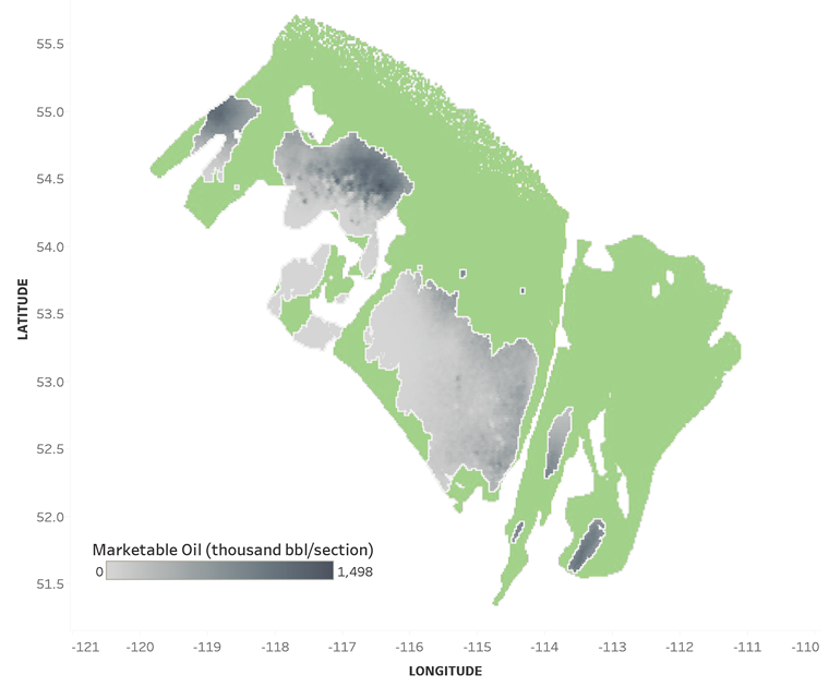
Description:
This map shows the concentration of Duvernay Shale marketable oil across the study area. The marketable oil is almost entirely found in the Duvernay Shale's southwest half, with most of that concentrated towards the basin's northwest corner and the basin's far southeast.
Figure A3. Map of the Duvernay Shale’s marketable NGLs (imperial units only). The green area of the map was excluded, because it fell below one or more of the study’s geological cut offs.
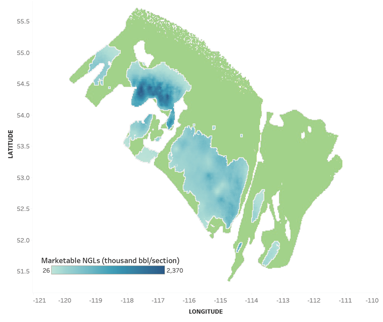
Description:
This map shows the concentration of Duvernay Shale marketable NGLs across the study area. The marketable NGLs are almost entirely found in the Duvernay Shale's southwest half, with most of that concentrated in the Duvernay Shale basin's northwest quarter.
Appendix B: Detailed Methods
Key Assumptions
- The oil and gas resource is considered to be a resource play, where the hydrocarbons are pervasively distributed through the geologically defined area. Thus, the chance of success at discovering hydrocarbons with a well is 100%.
- The estimated ultimate recoveries (EURs) of wells are based on existing technology, current trends in development, and limited production. Recoveries and levels of development could be different in the future as technology advances and the play matures.
Stratigraphy and Study Area
Stratigraphic intervals and Play Areas
The Duvernay Shale was treated as a single reservoir with no internal subdivisions, while its geographic extent was treated as two play areas, the East Shale Basin and the West Shale Basin. The study area was broken down into tractsFootnote 16 of approximately one-square mile in size. Some tracts were excluded from the analysis because they were considered unlikely to be developed; such as where the Duvernay Shale is less than 10 m thick, is underpressured, where its mapped in-place gas contents are less than 50 m³ of volume per m² of area, and where oil contents were more than 2000 barrels per million cubic feet of gas (i.e., there is too little gas in the reservoir to help drive the oil out). Only 27 819 km² of the full 108 244 km² assessed by the AGS for in-place resources (or 10 803 of the study area’s 42 012 square-mile tracts) were included after these criteria were applied (Figure B1).
Estimating Duvernay EURs
Reservoir indexing
The AGS mapped in-place raw natural gas, crude oil (including field condensate), and NGL volumes for the Duvernay Shale in a separate assessment.Footnote 17 To determine these volumes, the AGS mapped the Duvernay Shale’s geology, including net pay, pressure, and porosity. These data were extracted for every tract in the Duvernay study area. “Index” tracts in Kaybob (S22-T62-R21-MW5) and in Joffre (22-40-27-MW4) were chosen in the prospective parts of the West and East Shale Basins, respectively. Thus, every other tract could have their mapped net pays, pressures, and porosities compared to the values of the index tracts in their respective basins. In other words, each tract’s reservoir quality would be known relative to the index tract, such that worse tracts would have relative reservoir qualities of less than one, and better tracts would have relative reservoir qualities greater than one.
Figure B1. Duvernay Shale study area and assessed study area
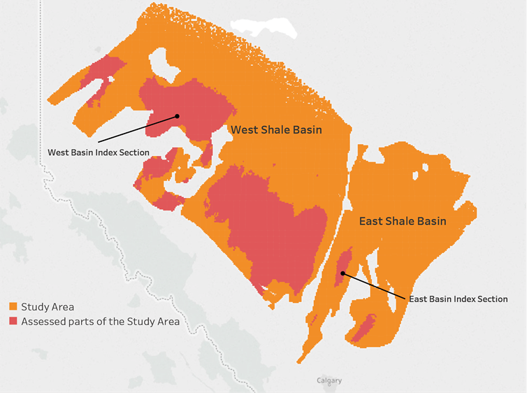
Description:
This map shows the study area, as well as what areas were assessed and what were excluded because of geological cutoffs. The southeast third of the Duvernay Shale basin is called the East Shale Basin and the northwest two-thirds is called the West Shale Basin. Most of the assessed area is located in the southwest half of the West Shale Basin while only three small parts of the East Shale Basin were assessed. This figure also shows the locations of the two index sections used for the assessment.
Production Data Gathering
Monthly production data from Duvernay shale gas and shale oil wells were gathered. Gas wells whose field condensate production was mathematically recombined with their gas production to meet AER reporting regulations were excluded, because it wasn’t possible to determine their separate liquid and gas streams (see also the AER’s Duvernay Reserves and Resources ReportFootnote 18). Therefore, the only gas wells used were those with either a full history of gas and field condensate production, or a limited history where the time series could be truncated at the last field condensate production reported. Duvernay shale oil wells always had two reported streams.
The selection of wells was also limited to those with a steady decline on the log-log plot of production versus time (i.e., a clear indication that the wells were in transient flow), such that the data could be confidently regressed. Some wells were excluded because of operational issues. In all, 90 gas wells and 19 oil wells were initially included in the analysis.
Decline Curve Analysis
Decline curve analysis was used to project the gas and field condensate production for each gas well, and crude oil and gas production for each oil well, assuming a well’s lifetime was 30 years. The decline curve analysis was two-stage. The first stage was transient flowFootnote 19, which was assumed to last 144 months (no Duvernay well currently shows signs of boundary-dominated flow even after 6 years of production, so 144 months was arbitrarily chosen as transient flow’s duration). Transient flow was followed by boundary-dominated flow for the remainder of the well’s life.
Each well was also analysed twice: 1) for main commodities (i.e., gas in gas wells and oil in oil wells); and 2) for energy-equivalent volumes, because rates of associated production like field condensate and associated gas were often too volatile to model alone. To determine the volumes of associated production, the main commodity production curves were subtracted from the energy-equivalent production curves and the result converted back to appropriate volumetric units assuming 5.8 thousand cubic feet of gas in a barrel of oil or field condensate.
Transient flow was modeled by identifying steady declines on log-log plots of historical production versus time and regressing them with DuongFootnote 20, Arps hyperbolicFootnote 21, and Long Duration Linear FlowFootnote 22 models. Regressed fits were then projected to the assumed start of boundary-dominated flow, or 144 months. It was assumed that initial production for boundary-dominated flow was the last projected production of transient flow, and that the initial, annual decline was 10%. The Arps b exponent was assumed to be 0.5 for gas production and barrel-of-oil-equivalent production, and 0.33 for oil production and gas-equivalent production. The 3 projections for each well’s gas production were then averaged and the same done to the 3 projections of liquid production.
For the rest of the analysis, field condensate was assumed to be crude oil. Each well’s monthly oil and gas production were combined to become barrels of oil equivalent (BOE). Monthly production of oil and gas were grouped to determine how the liquid fraction of monthly BOE production might evolve, because oil-to-gas ratios typically fall over time in producing wells.
Indexing Production Curves
Because each Duvernay well has a different length for their horizontal legs (ranging from less than 1 km to more than 2 km), each well’s BOE production was adjusted to a single kilometre of horizontal leg drilled so wells could be better compared to one another. Each well’s adjusted BOE production was further adjusted by its local reservoir quality (relative to the index tract of the basins the wells belonged to) to determine how they might perform if they were located at the index tracts.
The adjusted BOEs were then batched by basin and by well vintage to see if well performance improved over time. In the West Basin, a trend emerged from 2013 to 2016 (Figure B2). Thus, West Basin BOEs were adjusted to 2016 levels using the relationship between vintage year and average EUR while West Basin wells from prior to 2013 were excluded from the analysis (leaving a total of 88 wells used from the West Basin). There were too few wells in the East Shale Basin (a total of 8) to have confidence in any trends, however, so no East Basin wells were normalized relative to well vintage. The wells were then gathered to create index wells for the index tracts of each basin (Figure B3).
Figure B2. West Basin well EURs as batched by well vintage
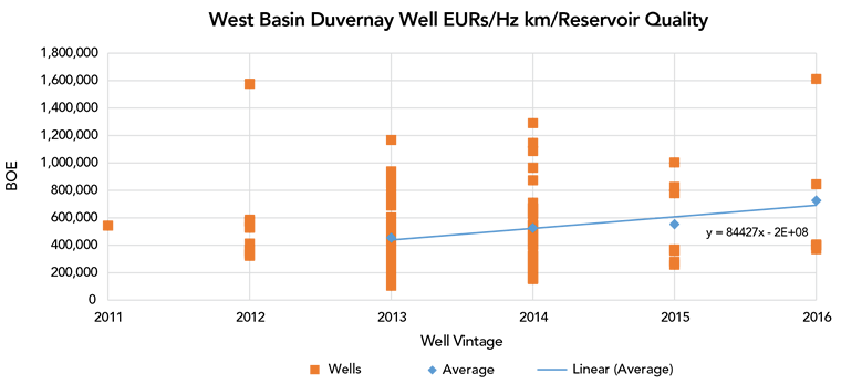
Description:
This graph shows the expected, ulitimate recoveries of Duvernay Shale wells as indexed to reservoir quality and length of horizontal legs. The wells are batched by year and, while there is considerable scatter in the results, expected recoveries appear to be increasing in newer wells versus older wells.
Figure B3. Duvernay Shale index-well type curves, historical and projected, as adjusted to km of horizontal leg length, relative reservoir quality, and well vintage.
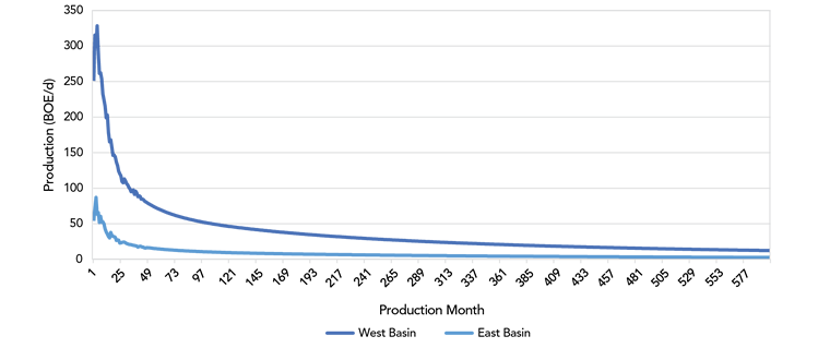
Description:
This graph shows the West Basin and East Basin production type curves as indexed to horizontal-leg length, reservoir quality, and well vintage. The West Basin's type curve peaks at about 325 BOE/d in month 4 before quickly declining to less than 100 BOE/d in 3 years and less than 50 BOE/d in 10 years, more gradually declining thereafter. The East Basin's type curve peaks at 87 BOE/d in month 3 before declining to 20 BOE/d in 3 years time and to 10 BOE/d in 10 years time, more gradually declining thereafter.
Modeling Raw Estimated EUR per Tract
The ranges of potential BOE EURs for the index well at the index sections were modeled using a lognormal distribution (Figure B4).
Figure B4. Statistical and modeled distributions of a) West Basin Duvernay Shale EURs; and b) East Basin Duvernay Shale EURs.
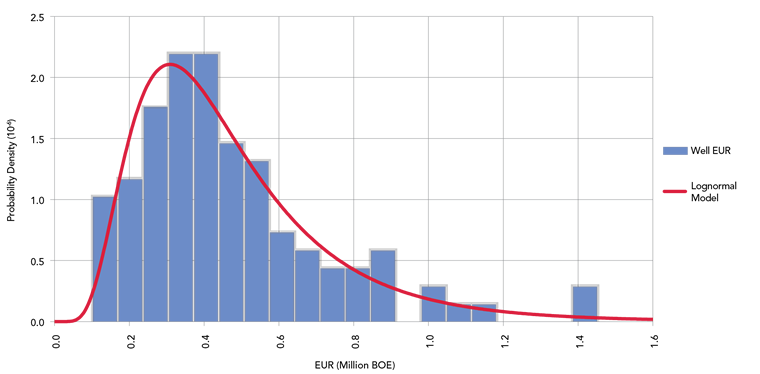
Description:
This graph shows the statistical and modeled distribution of Duvernay Shale well EURs. The data shows West Basin well EURs as small as about 0.1 million BOE and as large as about 1.4 million BOE, with a peak in likelihood at about 0.35 million BOE.
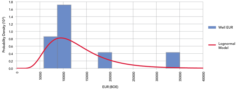
Description:
This graph shows the statistical and modeled distribution of Duvernay Shale well EURs. The data shows East Basin well EURs as small as about 70 000 BOE and as large as about 335 000 BOE, with a peak in likelihood at about 190 000 BOE.
To determine each tract’s BOE EUR, it was assumed that 5 horizontal wells with horizontal leg lengths of 1.6 km were required to fully develop a tract. The modeled EUR distributions of the index sections were then applied to every tract in their respective shale basins, adjusting them by local, relative reservoir quality. A Monte Carlo simulation of 1 000 iterations was run to determine the study area’s total low (P10) and high (P90) EURs. The expected EURs of tracts—which add together to become the study area’s expected EUR—were based on the statistical average of their respective basin’s index well and adjusted to local reservoir quality.
Estimated BOE EURs for each tract were divided into recoverable raw gas and recoverable oil as based on: 1) the initial oil and gas fractions at each tract; and 2) how the oil fraction evolves over the life of a well.
Estimating Tract Marketable EURs
Marketable oil in a tract was assumed to be the recoverable oil. Marketable NGLs in a tract were estimated from the local NGL-to-gas ratio mapped by the AGS as applied to the tract’s recoverable raw gas. Ethane, propane, butane, and pentane plus components were determined from how their fractions change depending on total NGL fraction of the raw gas in Duvernay Shale gas analyses. Gas-plant recoveries were assumed to be 60% for ethane, 75% for propane, 90% for butane, and 100% for pentanes plus.
A tract’s recoverable raw gas was converted to wellsite gas by subtracting 1% of production for wellsite fuel gas. Wellsite gas was converted to dry gas by subtracting marketable NGLs and a small fraction (0.5%) of non-hydrocarbon gas impurities. Dry gas was converted to marketable gas by subtracting 2% for gas-processing fuel and another 1% for pipeline fuel gas so it could be shipped to the NOVA Inventory Transfer pricing point (NIT).
Appendix C: Data
- Date modified: